Why RLE?#

Conceptually, a binary mask is a grid of 0s and 1s. But the same mask can be stored in memory in different ways, depending on what tradeoffs we want.

A dense array stores every pixel. A 1920×1080 mask takes 2 MB this way. But we might want to save space, so we could instead store it as a polygon, that is, just the vertices along the boundary. This is compact, but operations get messy. Intersecting two polygons, for example, is a notoriously hairy algorithm.

Luckily there is a representation that works well for natural inputs, saves storage and often speeds up processing. This is what this library is about: run-length encoding.

1D RLE#

As the name says, we encode the lengths of runs of identical values. Let’s see it first in 1D. Here is a binary sequence:

0 0 0 1 1 1 1 1 0 0

Instead of storing 10 values, we store the run lengths: 3, 5, 2. Three zeros, then five ones, then two zeros. We always start with the count of zeros, so we don’t need to store which value each run has.

From 2D to 1D#

A 2D mask is a grid of pixels. To apply RLE, we first flatten it into a 1D sequence. We could do this row by row. In fact, run-length ideas go back to early scanline displays like CRTs, which refreshed the image row by row, so encoding runs along scanlines was a natural fit for the hardware. But this library (and the COCO dataset format) uses column-major order: we go down the first column, then the second, and so on. We could also snake around in a zig-zag pattern if we wanted. It’s all about convention and ease of implementing the algorithms. Here we go column by column.

For example, a 4×4 mask:

Flattened column-wise becomes:

0 0 0 0 | 0 0 0 0 | 1 1 1 0 | 1 1 1 0

Which encodes as: 8, 3, 1, 3, 1. Eight zeros, three ones, one zero, three ones, one zero.

Perimeter, not area#

Why does this save space exactly? Does it always? It helps with intuition to look at a circle:

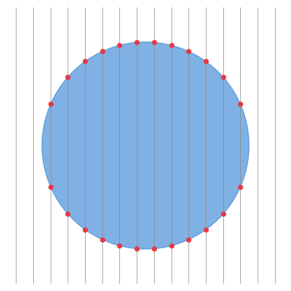
Think of scanning down each column. Every time we cross the boundary of the shape, we start a new run. Each column crosses the boundary about twice (in and out). The total number of boundary crossings across all columns is roughly the perimeter.

The number of runs is proportional to the perimeter of the shape, not its area. This is why RLE works well for “blobby” shapes. A solid disk has area proportional to r², but perimeter proportional to r. Double the radius, quadruple the pixels, but only double the storage. In other words, the storage roughly grows with the square root of the number of pixels.

Vertical edges are lucky: a straight vertical boundary adds only 2 runs, at the top and bottom. But natural masks tend to be smooth, so we usually don’t get this bonus. What matters is the sqrt.

When RLE hurts#

RLE assumes the mask has structure. If the mask looks like salt-and-pepper noise or a dense checkerboard, every pixel is a boundary crossing. Storage blows up to the size of a dense array or worse, and operations become slower than just working with pixels directly.

Know your data. If your masks are segmentation outputs, medical images, or anything with solid regions, RLE will serve you well. If they’re fine-grained textures or random noise, stick with dense arrays.

Fast, not just small#

RLE can also save processing time. On a dense array, every pixel must be touched. But many operations on RLE are proportional to the number of runs, not the number of pixels.

Boolean operations like union and intersection can merge two run sequences in a single pass, skipping over uniform regions where neither mask changes. Morphological operations like erosion work column by column, shifting runs up or down. Cropping is just adjusting run offsets. None of these need to decode the mask to a dense array first.

Since the number of runs grows with the perimeter, we get the same sqrt benefit for speed as we do for storage.

However, some algorithms can be tedious to express in a way that is tailored to RLE. The rest of these pages will discuss how it can be done.